How To Draw Capital Market Line In R

past Jonathan Regenstein

In a previous postal service, we covered how to calculate CAPM beta for our usual portfolio consisting of:

          + SPY (S&P500 fund) weighted 25% + EFA (a non-Usa equities fund) weighted 25% + IJS (a small-cap value fund) weighted 20% + EEM (an emerging-mkts fund) weighted 20% + AGG (a bond fund) weighted 10%        

Today, nosotros volition move on to visualizing the CAPM beta and explore some ggplot and highcharter functionality, along with the broom packet.

Before we can practice any of this CAPM work, we need to summate the portfolio returns, covered in this post, and then calculate the CAPM beta for the portfolio and the individual assets covered in this post.

I will not present that lawmaking or logic again but we will utilize four information objects from that previous work:

          + portfolio_returns_tq_rebalanced_monthly (a tibble of portfolio monthly returns) + market_returns_tidy (a tibble of SP500 monthly returns) + beta_dplyr_byhand (a tibble of market betas for our 5 individual assets) + asset_returns_long (a tibble of returns for our five individual assets)        

Let'southward get to it.

Visualizing the Human relationship between Portfolio Returns, Risk and Market Returns

The CAPM beta number is telling us nearly the linear relationship between our portfolio returns and the market returns. It's also telling u.s. nigh the riskiness of our portfolio - how volatile the portfolio is relative to the market. Earlier nosotros get to beta itself, permit'southward take a look at expected monthly returns of our avails scattered confronting monthly risk of our private assets.

            library(tidyquant) library(tidyverse) library(timetk) library(tibbletime) library(scales)  # This theme_update will middle your ggplot titles theme_update(plot.title = element_text(hjust = 0.five))  asset_returns_long %>%    group_by(asset) %>%    summarise(expected_return = mean(returns),             stand_dev = sd(returns)) %>%    ggplot(aes(x = stand_dev, y = expected_return, color = asset)) +   geom_point(size = 2) +   ylab("expected return") +   xlab("standard deviation") +   ggtitle("Expected Monthly Returns v. Risk") +   scale_y_continuous(characterization = office(10){ paste0(10, "%")})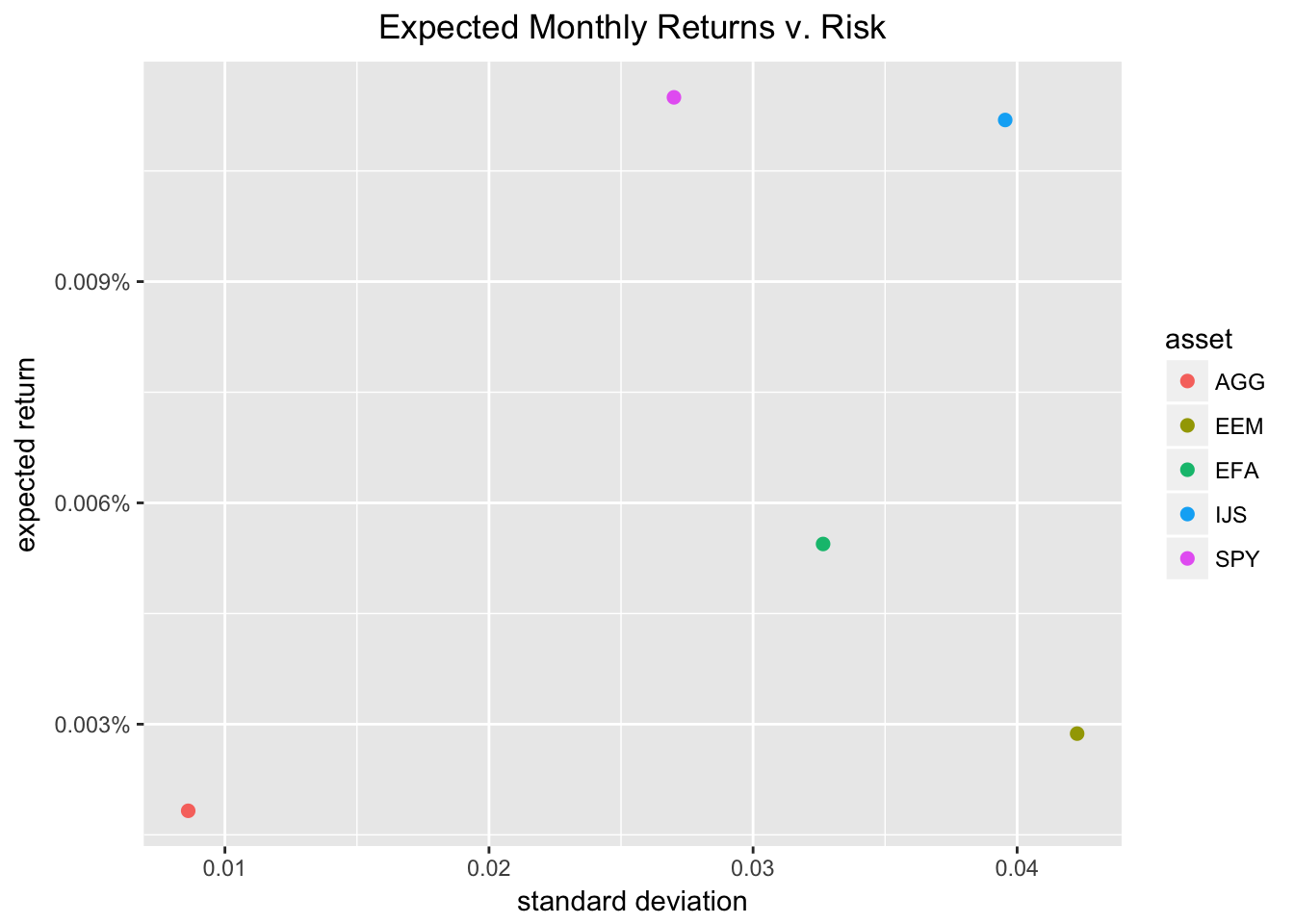                      

Where does our portfolio fit on this scatter plot? Allow's add it to the ggplot() flow with geom_point(aes(ten = sd(portfolio_returns_tq_rebalanced_monthly$returns), y = mean(portfolio_returns_tq_rebalanced_monthly$returns)), color = "cornflowerblue", size = 3).

            asset_returns_long %>%    group_by(asset) %>%    summarise(expected_return = hateful(returns),             stand_dev = sd(returns)) %>%    ggplot(aes(x = stand_dev, y = expected_return, color = asset)) +   geom_point(size = ii) +   geom_point(aes(x = sd(portfolio_returns_tq_rebalanced_monthly$returns),                    y = mean(portfolio_returns_tq_rebalanced_monthly$returns)),               colour = "cornflowerblue",               size = iii) +   geom_text(             aes(x = sd(portfolio_returns_tq_rebalanced_monthly$returns) * 1.09,                  y = mean(portfolio_returns_tq_rebalanced_monthly$returns),                  characterization = "portfolio")) +   ylab("expected return") +   xlab("standard deviation") +   ggtitle("Expected Monthly Returns v. Run a risk") +   scale_y_continuous(labels = office(10){ paste0(x, "%")})                      

Our portfolio return/adventure looks all right, though the SP500 has a college expected render for merely a flake more take a chance. Information technology's been tough to beat the marketplace the last v years. EEM and EFA accept a higher risk and lower expected return (no rational investor wants that!) and IJS has a higher risk and a higher expected return (some rational investors exercise want that!).

In general, the scatter is providing some return-risk context for our portfolio. It's not straight role of CAPM, merely I like to start hither to go far the render-risk mindset.

Next, let'south turn to CAPM more directly and visualize the relationship betwixt our portfolio and the market with a scatter plot of market returns on the 10-axis and portfolio returns on the y-axis. First, we will add the market place returns to our portfolio tibble by calling mutate(market_returns = market_returns_tidy$returns). So, we set our x- and y-axis with ggplot(aes(x = market_returns, y = returns)).

            portfolio_returns_tq_rebalanced_monthly %>%    mutate(market_returns = market_returns_tidy$returns) %>%    ggplot(aes(10 = market_returns, y = returns)) +    geom_point(color = "cornflowerblue") +   ylab("portfolio returns") +   xlab("market returns") +   ggtitle("Scatterplot of portfolio returns 5. market returns")          

This scatter plot is communicating the same stiff linear relationship as our numeric beta calculation from the previous post. We can add a uncomplicated regression line to it with geom_smooth(method = "lm", se = FALSE, color = "green", size = .five).

            portfolio_returns_tq_rebalanced_monthly %>%    mutate(market_returns = market_returns_tidy$returns) %>%    ggplot(aes(x = market_returns, y = returns)) +    geom_point(color = "cornflowerblue") +   geom_smooth(method = "lm", se = FALSE, color = "green", size = .five) +   ylab("portfolio returns") +   xlab("market place returns") +    ggtitle("Scatterplot with regression line")          

The light-green line is produced by the phone call to geom_smooth(method = 'lm'). Under the hood, ggplot fits a linear model of the human relationship between market returns and portfolio returns. The gradient of that greenish line is the CAPM beta that we calculated earlier. To ostend that we can add a line to the scatter that has a slope equal to our beta calculation and a y-intercept equal to what I labeled as alpha in the beta_dplyr_byhand object.

To add the line, we invoke geom_abline(aes(intercept = beta_dplyr_byhand$approximate[1], slope = beta_dplyr_byhand$estimate[ii]), colour = "regal").

            portfolio_returns_tq_rebalanced_monthly %>%    mutate(market_returns = market_returns_tidy$returns) %>%    ggplot(aes(ten = market_returns, y = returns)) +    geom_point(color = "cornflowerblue") +   geom_abline(aes(     intercept = beta_dplyr_byhand$estimate[one],      slope = beta_dplyr_byhand$approximate[2]),      color = "majestic",     size = .five) +   ylab("portfolio returns") +   xlab("market returns") +   ggtitle("Scatterplot with paw calculated gradient")          

We tin can plot both lines simultaneously to ostend to ourselves that they are the same - they should be right on top of each other but the purple line, our manual abline, extends into infinity so, we should run into information technology start where the green line ends.

            portfolio_returns_tq_rebalanced_monthly %>%    mutate(market_returns = market_returns_tidy$returns) %>%    ggplot(aes(ten = market_returns, y = returns)) +    geom_point(colour = "cornflowerblue") +   geom_abline(aes(     intercept = beta_dplyr_byhand$gauge[ane],      slope = beta_dplyr_byhand$estimate[2]),      color = "purple",      size = .five) +   geom_smooth(method = "lm", se = FALSE, colour = "light-green", size = .5) +   ylab("portfolio returns") +   xlab("market place returns") +   ggtitle("Compare CAPM beta line to regression line")          

All right, that seems to visually ostend (or strongly back up) that the fitted line calculated by ggplot and geom_smooth() has a gradient equal to the beta nosotros calculated ourselves. Why did we go through this practise? Well, CAPM beta is a bit "jargony". Since we need to map that jargon over to the globe of linear modeling, information technology's a useful do to consider how jargon reduces to information scientific discipline concepts. This isn't a particularly complicated scrap of jargon, but it's good practice to get in the habit of reducing jargon.

A Chip More on Linear Regression: Augmenting Our Data

Before concluding our analysis of CAPM beta, let'due south explore the broaden() function from broom and how it helps to create a few more interesting visualizations.

The lawmaking clamper below starts with model results from lm(returns ~ market_returns_tidy$returns...), which is regressing our portfolio returns on the market returns. We store the results in a list-column called chosen model. Adjacent, nosotros call augment(model) which volition add predicted values to the original data ready and return a tibble.

Those predicted values will be in the .fitted cavalcade. For some reason, the date column gets dropped. It's nice to have this for visualizations so we will add it back in with mutate(date = portfolio_returns_tq_rebalanced_monthly$engagement).

            library(broom)  portfolio_model_augmented <-  portfolio_returns_tq_rebalanced_monthly %>%    practise(model = lm(returns ~ market_returns_tidy$returns, information = .))%>%    augment(model) %>%    mutate(date = portfolio_returns_tq_rebalanced_monthly$date)  head(portfolio_model_augmented)          

            ##         returns market_returns_tidy.returns      .fitted     .se.fit ## 1 -0.0008696132                  0.01267837  0.008294282 0.001431288 ## 2  0.0186624378                  0.03726809  0.030451319 0.001984645 ## 3  0.0206248830                  0.01903021  0.014017731 0.001485410 ## iv -0.0053529692                  0.02333503  0.017896670 0.001563417 ## v -0.0229487590                 -0.01343411 -0.015234859 0.001953853 ## half-dozen  0.0411705787                  0.05038580  0.042271276 0.002521506 ##         .resid       .lid     .sigma     .cooksd .std.resid       date ## 1 -0.009163896 0.01698211 0.01101184 0.006116973 -0.8415272 2022-02-28 ## 2 -0.011788881 0.03265148 0.01096452 0.020099701 -1.0913142 2022-03-28 ## 3  0.006607152 0.01829069 0.01104500 0.003434000  0.6071438 2022-04-thirty ## four -0.023249640 0.02026222 0.01062704 0.047294116 -ii.1386022 2022-05-31 ## five -0.007713900 0.03164618 0.01103127 0.008323550 -0.7137165 2022-06-28 ## 6 -0.001100697 0.05270569 0.01107986 0.000294938 -0.1029661 2022-07-31          

Let'south use ggplot() to see how well the fitted return values match the actual return values.

            portfolio_model_augmented %>%    ggplot(aes(ten = date)) +    geom_line(aes(y = returns, colour = "actual returns")) +    geom_line(aes(y = .fitted, color = "fitted returns")) +   scale_colour_manual("",                        values = c("fitted returns" = "green",                                   "actual returns" = "cornflowerblue")) +   xlab("date") +    ggtitle("Fitted versus bodily returns")          

Those monthly returns and fitted values seem to track well. Allow'southward catechumen both bodily returns and fitted returns to the growth of a dollar and run the aforementioned comparing. This isn't a traditional way to visualize actual versus fitted, but it's still useful.

            portfolio_model_augmented %>%   mutate(actual_growth = cumprod(one + returns),           fitted_growth = cumprod(1 + .fitted)) %>%    ggplot(aes(x = date)) +    geom_line(aes(y = actual_growth, colour = "actual growth")) +    geom_line(aes(y = fitted_growth, color = "fitted growth")) +   xlab("date") +   ylab("bodily and fitted growth") +    ggtitle("Growth of a dollar: actual v. fitted") +   scale_x_date(breaks = pretty_breaks(n = 8)) +   scale_y_continuous(labels = dollar) +   scale_colour_manual("",                        values = c("fitted growth" = "light-green",                                   "actual growth" = "cornflowerblue"))                      

Our fitted growth tracks our actual growth well, though the actual growth is lower than predicted for most of the v yr history.

To Highcharter!

A nice side benefit of augment() is that information technology allows us to create an interesting highcharter object that replicates our scatter + regression ggplot from earlier.

Starting time, let's build the base scatter plot of portfolio returns, which are housed in portfolio_model_augmented$returns, against market returns, which are housed in portfolio_model_augmented$market_returns_tidy.returns.

            library(highcharter)  highchart() %>%    hc_title(text = "Portfolio v. Market Returns") %>%   hc_add_series_scatter(round(portfolio_model_augmented$returns, 4),                          round(portfolio_model_augmented$market_returns_tidy.returns, 4)) %>%   hc_xAxis(title = list(text = "Market Returns")) %>%    hc_yAxis(title = listing(text = "Portfolio Returns"))          

That looks proficient; but hover over i of the points. If you're like me, yous volition desperately wish that the date of the observation were being displayed. Allow'southward add that date display functionality.

First, nosotros need to supply the date observations, so we will add together a date variable with hc_add_series_scatter(..., engagement = portfolio_returns_tq_rebalanced_monthly$engagement). And so, we desire the tool tip to pick up and display that variable. That is done with hc_tooltip(formatter = JS("function(){render ('port return: ' + this.y + ' <br> mkt render: ' + this.x + ' <br> date: ' + this.indicate.date)}")). We are creating a custom tool tip function to selection up the date. Run the code chunk beneath and hover over a bespeak.

            highchart() %>%    hc_title(text = "Portfolio v. Marketplace Returns") %>%   hc_add_series_scatter(circular(portfolio_model_augmented$returns, 4),                          round(portfolio_model_augmented$market_returns_tidy.returns, 4),                          date = portfolio_model_augmented$date) %>%   hc_xAxis(title = list(text = "Market Returns")) %>%    hc_yAxis(title = list(text = "Portfolio Returns")) %>%    hc_tooltip(formatter = JS("function(){                             return ('port return: ' + this.y + ' <br> mkt return: ' + this.10 +                               ' <br> appointment: ' + this.point.date)}"))          

I was curious nigh the most negative reading in the lesser left, and this new tool tip makes it easy to see that it occurred in August of 2022.

Finally, allow's add together the regression line.

To do that, we need to supply ten and y coordinates to highcharter and specify that we desire to add together a line instead of more scatter points. We take the ten and y coordinates for our fitted regression line because we added them with the broaden() office. The x's are the marketplace returns and the y'southward are the fitted values. Nosotros add this chemical element to our code menstruum with hc_add_series(portfolio_model_augmented, type = "line", hcaes(ten = market_returns_tidy.returns, y = .fitted), proper name = "CAPM Beta = Regression Slope")

            highchart() %>%    hc_title(text = "Scatter with Regression Line") %>%    hc_add_series(portfolio_model_augmented,                  blazon = "scatter",                  hcaes(10 = circular(market_returns_tidy.returns, 4),                        y = circular(returns, 4),                       engagement = appointment),                  name = "Returns") %>%   hc_add_series(portfolio_model_augmented,                  type = "line",                  hcaes(x = market_returns_tidy.returns, y = .fitted),                  proper name = "CAPM Beta = Regression Slope") %>%    hc_xAxis(title = list(text = "Market Returns")) %>%    hc_yAxis(title = listing(text = "Portfolio Returns")) %>%    hc_tooltip(formatter = JS("function(){                             render ('port render: ' + this.y + ' <br> mkt return: ' + this.x +                               ' <br> appointment: ' + this.point.date)}"))          

That's all for today and thanks for reading.

Source: https://rviews.rstudio.com/2018/03/02/capm-and-visualization/

Posted by: caballeroarriess.blogspot.com

Share this post